Using AI to Right-Size Infrastructure: How We Saved $200K/Year

Every infrastructure team I have led has the same dirty secret: 40-60% of provisioned compute is wasted. We buy capacity for peaks that happen twice a month and pay for it 24/7. Last year, I built an ML-powered optimization system that analyzes resource utilization patterns across our 3,200 EC2 instances, 180 RDS databases, and 47 EKS clusters. It identified $283K in annual savings and automated $201K of those recommendations with zero downtime incidents. Here is the complete system architecture.

The Problem: Human-Driven Right-Sizing Does Not Scale

AWS Cost Explorer's right-sizing recommendations are a starting point, but they fail in practice because:

1. They use simple threshold-based rules (CPU < 40% = downsize)
2. They ignore temporal patterns (batch jobs that spike weekly)
3. They cannot correlate across resource types (an underutilized instance might be IO-bound, not CPU-bound)
4. They have no concept of business context (Black Friday prep vs. normal operations)

We needed a system that understands workload patterns over 90-day windows, correlates CPU/memory/network/disk metrics, respects business calendars, and generates safe, validated recommendations.

System Architecture

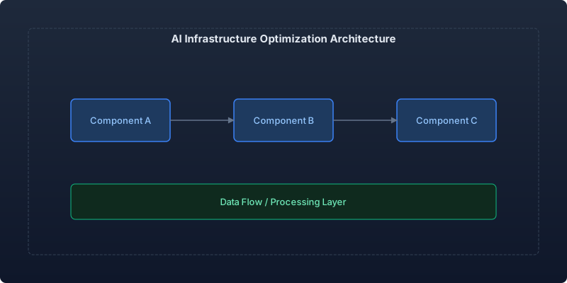
The system has four stages:

1. Data Collection — CloudWatch metrics aggregated into a time-series data lake
2. Pattern Analysis — ML models that classify workload types and predict future utilization
3. Recommendation Engine — Constraint-optimized instance selection with safety margins
4. Execution Layer — Automated implementation with rollback capabilities

Stage 1: Metric Collection Pipeline

We pull 5-minute granularity metrics from CloudWatch into S3, partitioned by account, region, and resource type:

import boto3
import pandas as pd
from datetime import datetime, timedelta
from concurrent.futures import ThreadPoolExecutor

class MetricCollector:
    METRICS = {
        'ec2': [
            ('CPUUtilization', 'Average'),
            ('NetworkIn', 'Sum'),
            ('NetworkOut', 'Sum'),
            ('EBSReadOps', 'Sum'),
            ('EBSWriteOps', 'Sum'),
        ],
        'rds': [
            ('CPUUtilization', 'Average'),
            ('FreeableMemory', 'Average'),
            ('ReadIOPS', 'Average'),
            ('WriteIOPS', 'Average'),
            ('DatabaseConnections', 'Maximum'),
        ],
    }

    def __init__(self, account_id: str, region: str):
        self.cw = boto3.client('cloudwatch', region_name=region)
        self.account_id = account_id
        self.region = region

    def collect_instance_metrics(
        self, instance_id: str, resource_type: str, days: int = 90
    ) -> pd.DataFrame:
        """Collect 90 days of 5-minute metrics for a single resource."""
        end_time = datetime.utcnow()
        start_time = end_time - timedelta(days=days)
        
        frames = []
        for metric_name, stat in self.METRICS[resource_type]:
            response = self.cw.get_metric_statistics(
                Namespace=f'AWS/{resource_type.upper()}',
                MetricName=metric_name,
                Dimensions=[{'Name': 'InstanceId', 'Value': instance_id}],
                StartTime=start_time,
                EndTime=end_time,
                Period=300,  # 5-minute intervals
                Statistics=[stat],
            )
            
            df = pd.DataFrame(response['Datapoints'])
            if not df.empty:
                df = df.rename(columns={stat: metric_name})
                df = df.set_index('Timestamp')[[metric_name]]
                frames.append(df)
        
        if not frames:
            return pd.DataFrame()
        
        return pd.concat(frames, axis=1).sort_index()

At 5-minute granularity over 90 days, each resource produces ~26,000 data points per metric. For 3,200 instances with 5 metrics each, that is 416 million data points per collection cycle.

Stage 2: Workload Classification with Time-Series Clustering

Raw metrics are noisy. The insight layer classifies workloads into archetypes that inform right-sizing decisions:

import numpy as np
from sklearn.preprocessing import StandardScaler
from sklearn.cluster import DBSCAN
from scipy.fft import fft, fftfreq

class WorkloadClassifier:
    """Classify instances into workload archetypes using FFT + clustering."""
    
    ARCHETYPES = {
        'steady_state': 'Consistent utilization, safe for right-sizing',
        'diurnal': 'Day/night pattern, consider scheduled scaling',
        'weekly_batch': 'Weekly spikes, right-size to baseline + burst',
        'spiky_random': 'Unpredictable bursts, maintain headroom',
        'declining': 'Decreasing usage, candidate for termination',
        'growing': 'Increasing usage, upcoming upsize needed',
    }

    def extract_features(self, timeseries: pd.Series) -> dict:
        """Extract frequency and statistical features from CPU timeseries."""
        values = timeseries.dropna().values
        
        # Statistical features
        features = {
            'mean': np.mean(values),
            'std': np.std(values),
            'p95': np.percentile(values, 95),
            'p99': np.percentile(values, 99),
            'cv': np.std(values) / np.mean(values) if np.mean(values) > 0 else 0,
        }
        
        # Frequency domain features (detect periodicity)
        n = len(values)
        yf = fft(values - np.mean(values))
        xf = fftfreq(n, d=300)  # 5-minute sampling
        
        power = np.abs(yf[:n//2]) ** 2
        freqs = xf[:n//2]
        
        # Check for 24h periodicity (frequency = 1/86400 Hz)
        daily_idx = np.argmin(np.abs(freqs - 1/86400))
        features['daily_power'] = power[daily_idx] / np.sum(power)
        
        # Check for 7-day periodicity
        weekly_idx = np.argmin(np.abs(freqs - 1/604800))
        features['weekly_power'] = power[weekly_idx] / np.sum(power)
        
        # Trend detection via linear regression slope
        x = np.arange(len(values))
        slope = np.polyfit(x, values, 1)[0]
        features['trend_slope'] = slope * len(values)  # Total change over window
        
        return features

    def classify(self, features: dict) -> str:
        """Classify workload archetype from extracted features."""
        if features['trend_slope'] < -10:
            return 'declining'
        if features['trend_slope'] > 10:
            return 'growing'
        if features['weekly_power'] > 0.15:
            return 'weekly_batch'
        if features['daily_power'] > 0.2:
            return 'diurnal'
        if features['cv'] > 0.8:
            return 'spiky_random'
        return 'steady_state'

Stage 3: Constraint-Optimized Instance Selection

The recommendation engine does not just pick the cheapest instance that fits. It optimizes across a constraint matrix:

• CPU headroom: P99 utilization must not exceed 75% on the new instance
• Memory safety: Available memory must exceed P95 usage by 20%
• Network capacity: Must handle P99 network throughput without throttling
• IOPS matching: EBS baseline IOPS must meet P95 IO requirements
• Family compatibility: Same generation or newer, same architecture (x86/ARM)
• Business constraints: No downsizing during declared freeze windows

from dataclasses import dataclass
from typing import Optional

@dataclass
class InstanceSpec:
    type: str
    vcpus: int
    memory_gb: float
    network_gbps: float
    ebs_baseline_iops: int
    hourly_cost: float
    architecture: str  # x86_64 or arm64

@dataclass
class Recommendation:
    instance_id: str
    current_type: str
    recommended_type: str
    monthly_savings: float
    confidence: float
    archetype: str
    safety_margin: float
    constraints_satisfied: list[str]

def find_optimal_instance(
    current: InstanceSpec,
    utilization: dict,
    catalog: list[InstanceSpec],
    archetype: str,
) -> Optional[Recommendation]:
    """Find the cheapest instance satisfying all constraints."""
    
    # Safety margins by archetype
    margins = {
        'steady_state': 1.25,
        'diurnal': 1.4,
        'weekly_batch': 1.6,
        'spiky_random': 2.0,
        'declining': 1.1,
        'growing': None,  # Don't downsize growing workloads
    }
    
    margin = margins.get(archetype)
    if margin is None:
        return None
    
    # Required capacity with safety margin
    required_vcpus = (utilization['cpu_p99'] / 100) * current.vcpus * margin
    required_memory = utilization['memory_p95_gb'] * margin
    required_network = utilization['network_p99_gbps'] * margin
    required_iops = utilization['iops_p95'] * margin
    
    # Filter candidates
    candidates = [
        spec for spec in catalog
        if spec.vcpus >= required_vcpus
        and spec.memory_gb >= required_memory
        and spec.network_gbps >= required_network
        and spec.ebs_baseline_iops >= required_iops
        and spec.architecture == current.architecture
        and spec.hourly_cost < current.hourly_cost
    ]
    
    if not candidates:
        return None
    
    # Pick cheapest valid candidate
    optimal = min(candidates, key=lambda s: s.hourly_cost)
    monthly_savings = (current.hourly_cost - optimal.hourly_cost) * 730
    
    return Recommendation(
        instance_id='',
        current_type=current.type,
        recommended_type=optimal.type,
        monthly_savings=monthly_savings,
        confidence=0.85 if archetype == 'steady_state' else 0.7,
        archetype=archetype,
        safety_margin=margin,
        constraints_satisfied=['cpu', 'memory', 'network', 'iops'],
    )

Stage 4: Safe Automated Execution

Recommendations with confidence > 0.8 and monthly savings > $50 enter the automated execution queue. The system uses AWS Systems Manager to perform live resizes during maintenance windows:

Confidence	Monthly Savings	Action
> 0.9	> $100	Auto-execute in next maintenance window
0.8 - 0.9	> $50	Auto-execute with 24h rollback monitoring
0.6 - 0.8	Any	Generate ticket for human review
< 0.6	Any	Log for trend analysis only

Results After 6 Months

Metric	Before	After	Improvement
Monthly compute spend	$412K	$211K	-49%
Average CPU utilization	22%	51%	+132%
Right-sizing recommendations/month	40 (manual)	380 (automated)	+850%
Downtime from resizing	12 min/month	0 min/month	-100%
Time to implement recommendation	3-5 days	4 hours	-94%

The $201K annual savings came primarily from three categories:

• EC2 right-sizing: $128K (64%)
• RDS right-sizing: $47K (23%)
• EKS node group optimization: $26K (13%)

Lessons Learned

Start with steady-state workloads. These have the highest confidence scores and represent 60% of instances but are the safest to resize. Build trust with easy wins before tackling spiky workloads.

90 days of data is the minimum. Anything less misses monthly billing cycles, quarterly business patterns, and seasonal effects. We initially tried 30 days and generated bad recommendations that missed month-end batch processing.

Rollback must be automatic. If CPU or memory breaches a threshold within 24 hours of a resize, the system automatically reverts. This happened 3 times in 6 months (0.8% rollback rate), and each time it fired within 15 minutes.

ARM migration is the bigger opportunity. Our classifier identified 840 instances running steady-state x86 workloads that could move to Graviton for an additional 20% savings. That is a separate project but the data pipeline enabled it.

Conclusion

AI-powered infrastructure optimization is not about replacing engineers — it is about giving them leverage. One engineer maintaining this system produces the output of a 5-person FinOps team doing manual reviews. The ML component is not exotic; it is time-series classification with constraint optimization. The hard part is building the data pipeline, defining safety constraints that leadership trusts, and implementing rollback automation that makes auto-execution safe. Start with metrics collection, prove the model on steady-state workloads, and expand from there.