Text Classification at Scale: Production Pipeline Guide

Text classification remains one of the most common NLP tasks in production systems. From routing customer support tickets to flagging policy violations, organizations process millions of text documents daily. Yet the gap between a fine-tuned model in a notebook and a reliable production pipeline is significant.

In this article, I break down the architecture, optimization techniques, and operational patterns that make text classification systems reliable at scale.

The Production Architecture

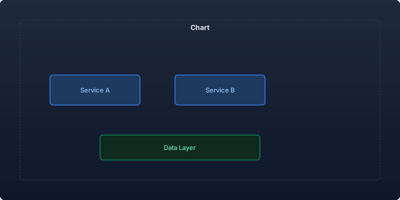
A production text classification pipeline consists of several interconnected components that must work in concert:

Component	Responsibility	Latency Budget
Input Preprocessing	Tokenization, normalization	< 5ms
Model Inference	Forward pass through transformer	< 50ms
Post-processing	Confidence thresholding, routing	< 2ms
Caching Layer	Deduplication, result storage	< 3ms
Monitoring	Drift detection, performance tracking	Async

The key insight is that inference is only one piece of the puzzle. The surrounding infrastructure determines whether your system handles 10 requests per second or 10,000.

Model Selection and Training

For production text classification, model choice directly impacts your infrastructure costs and latency profile. Here is how the most common architectures compare:

Model	Parameters	Inference (P95)	F1-Score (avg)	Cost/1M requests
DistilBERT	66M	12ms	0.89	$2.40
BERT-base	110M	23ms	0.91	$4.80
DeBERTa-v3-base	184M	38ms	0.93	$7.60
GPT-3.5 (API)	175B	890ms	0.92	$45.00

For most production use cases, DistilBERT or a similarly distilled model provides the best cost-performance tradeoff. The 2-point F1 improvement from larger models rarely justifies 3x the infrastructure cost.

Training Pipeline Implementation

Here is a production-ready training pipeline using Hugging Face Transformers:

import torch
from transformers import (
    AutoModelForSequenceClassification,
    AutoTokenizer,
    TrainingArguments,
    Trainer,
)
from datasets import load_dataset
from sklearn.metrics import classification_report
import wandb

class TextClassificationPipeline:
    def __init__(self, model_name: str, num_labels: int, max_length: int = 256):
        self.tokenizer = AutoTokenizer.from_pretrained(model_name)
        self.model = AutoModelForSequenceClassification.from_pretrained(
            model_name, num_labels=num_labels
        )
        self.max_length = max_length

    def preprocess(self, examples):
        return self.tokenizer(
            examples["text"],
            truncation=True,
            padding="max_length",
            max_length=self.max_length,
        )

    def train(self, train_dataset, eval_dataset, output_dir: str):
        training_args = TrainingArguments(
            output_dir=output_dir,
            num_train_epochs=3,
            per_device_train_batch_size=32,
            per_device_eval_batch_size=64,
            warmup_ratio=0.1,
            weight_decay=0.01,
            evaluation_strategy="steps",
            eval_steps=500,
            save_strategy="steps",
            save_steps=500,
            load_best_model_at_end=True,
            metric_for_best_model="f1_macro",
            fp16=torch.cuda.is_available(),
            report_to="wandb",
        )

        trainer = Trainer(
            model=self.model,
            args=training_args,
            train_dataset=train_dataset,
            eval_dataset=eval_dataset,
            compute_metrics=self._compute_metrics,
        )

        trainer.train()
        return trainer

    def _compute_metrics(self, eval_pred):
        predictions, labels = eval_pred
        preds = predictions.argmax(-1)
        report = classification_report(labels, preds, output_dict=True)
        return {
            "f1_macro": report["macro avg"]["f1-score"],
            "accuracy": report["accuracy"],
        }

Serving Infrastructure

For serving, I recommend a multi-tier caching strategy combined with dynamic batching:

from fastapi import FastAPI
from functools import lru_cache
import hashlib
import redis
import numpy as np
from optimum.onnxruntime import ORTModelForSequenceClassification

app = FastAPI()
redis_client = redis.Redis(host="localhost", port=6379, db=0)

class InferenceServer:
    def __init__(self, model_path: str):
        self.model = ORTModelForSequenceClassification.from_pretrained(model_path)
        self.tokenizer = AutoTokenizer.from_pretrained(model_path)

    def classify(self, text: str) -> dict:
        cache_key = hashlib.md5(text.encode()).hexdigest()

        # Check Redis cache first
        cached = redis_client.get(cache_key)
        if cached:
            return json.loads(cached)

        # Run inference
        inputs = self.tokenizer(
            text, return_tensors="pt", truncation=True, max_length=256
        )
        outputs = self.model(**inputs)
        probs = torch.softmax(outputs.logits, dim=-1)

        result = {
            "label": self.model.config.id2label[probs.argmax().item()],
            "confidence": probs.max().item(),
        }

        # Cache for 1 hour
        redis_client.setex(cache_key, 3600, json.dumps(result))
        return result

Performance Optimization

Converting to ONNX Runtime yields significant latency improvements:

Optimization	Latency (P50)	Latency (P95)	Throughput
PyTorch (FP32)	23ms	45ms	43 req/s
PyTorch (FP16)	14ms	28ms	71 req/s
ONNX Runtime	8ms	15ms	125 req/s
ONNX + Quantization (INT8)	5ms	9ms	200 req/s

The combination of ONNX export and INT8 quantization delivers a 4.6x throughput improvement with less than 1% accuracy degradation on most classification tasks.

Monitoring and Drift Detection

Production systems degrade silently. Implement distribution monitoring to catch data drift before it impacts business metrics:

from scipy.stats import ks_2samp
import numpy as np

class DriftDetector:
    def __init__(self, reference_predictions: np.ndarray, threshold: float = 0.05):
        self.reference = reference_predictions
        self.threshold = threshold
        self.window = []
        self.window_size = 1000

    def check(self, new_prediction: float) -> bool:
        self.window.append(new_prediction)
        if len(self.window) >= self.window_size:
            statistic, p_value = ks_2samp(self.reference, self.window)
            self.window = self.window[self.window_size // 2:]
            if p_value < self.threshold:
                self._alert(statistic, p_value)
                return True
        return False

    def _alert(self, statistic: float, p_value: float):
        # Send alert via PagerDuty, Slack, etc.
        print(f"DRIFT DETECTED: KS={statistic:.4f}, p={p_value:.6f}")

Deployment Patterns

For production deployments, I recommend the shadow deployment pattern for new model versions:

1. Shadow Mode (Week 1-2): New model runs alongside production, predictions logged but not served
2. Canary (Week 3): 5% of traffic routes to new model with real-time comparison
3. Gradual Rollout (Week 4): Increase to 25%, 50%, 100% if metrics hold
4. Rollback: Automated rollback if error rate exceeds threshold

Error Analysis and Continuous Improvement

Production text classification requires a systematic approach to error analysis. Track confusion patterns to identify where your model consistently fails:

Error Pattern	Frequency	Root Cause	Mitigation
Short text misclassification	18%	Insufficient context	Add context enrichment
Sarcasm/irony confusion	12%	Literal interpretation	Augment training data
Multi-label overlap	15%	Ambiguous categories	Refine taxonomy
Domain jargon failures	8%	OOV tokens	Domain-specific tokenizer
Cross-language mixing	5%	Monolingual model	Multilingual fine-tuning

Build a human review queue for low-confidence predictions (confidence < 0.7) and use those corrected labels as training data for the next model iteration. This feedback loop is what separates static models from continuously improving systems. In practice, a monthly retraining cadence with 2-5K new labeled examples maintains model freshness against evolving text distributions.

Key Takeaways

• Model selection matters less than you think. DistilBERT achieves 98% of BERT-large performance at 25% of the cost.
• ONNX Runtime + INT8 quantization delivers 4-5x throughput improvements with minimal accuracy loss.
• Cache aggressively. In most production workloads, 30-60% of inputs are duplicates or near-duplicates.
• Monitor distribution, not just accuracy. Data drift causes silent failures that business metrics only catch weeks later.
• Deploy incrementally. Shadow deployments eliminate surprise failures and give you confidence in new model versions.

The best text classification systems are not the ones with the highest F1 score in isolation. They are the systems that maintain consistent performance under real-world conditions while remaining cost-effective and operationally simple.