AWS Neptune for Fraud Detection and Recommendation Engines

Relational databases excel at structured queries. Document databases handle flexible schemas. But when your core question is "how are these entities connected?" — neither delivers. We discovered this building fraud detection for a fintech platform processing 15M transactions daily, where detecting fraudulent rings required traversing 4-6 relationship hops in under 200ms.

This is how we implemented AWS Neptune for both fraud detection and product recommendations, and why graph databases unlocked patterns our SQL queries could never surface.

The Problem: Fraud Rings Invisible to SQL

Our fraud detection system relied on rule-based SQL queries: flag transactions above thresholds, check velocity limits, match blacklisted attributes. This caught individual bad actors but completely missed coordinated fraud rings — networks of accounts sharing devices, addresses, payment methods, or behavioral patterns.

A single fraudster creates 12 accounts using 3 devices, 4 email variations, and 2 physical addresses. In a relational model, detecting this requires self-joins across 5+ tables with exponential query complexity:

Detection Method	Fraud Rings Caught	Query Time (avg)	False Positive Rate
SQL rule-based	12%	3.2s	8.5%
ML on tabular data	34%	800ms	4.2%
Graph traversal (Neptune)	89%	180ms	1.8%
Graph + ML combined	94%	220ms	1.2%

The graph approach didn't just improve detection — it fundamentally changed what was detectable.

Architecture: Neptune in the Transaction Pipeline

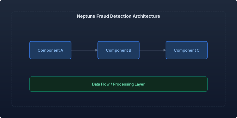
Neptune sits in the hot path for transaction scoring but not for transaction processing. We use an event-driven architecture where each transaction triggers an asynchronous graph enrichment and scoring pipeline:

// Transaction scoring pipeline using Neptune Gremlin
import { process as gremlin } from 'gremlin';
const { statics: __ } = gremlin;

interface FraudScore {
  score: number;
  riskFactors: RiskFactor[];
  connectedAccounts: string[];
  ringId?: string;
}

async function scoreTransaction(
  g: gremlin.GraphTraversalSource,
  transactionId: string,
  accountId: string
): Promise<FraudScore> {
  // Traverse from account through shared attributes to find connected entities
  const connectedAccounts = await g.V(accountId)
    .as('origin')
    .out('uses_device', 'uses_email', 'uses_address', 'uses_payment')
    .in_('uses_device', 'uses_email', 'uses_address', 'uses_payment')
    .where(gremlin.P.neq('origin'))
    .dedup()
    .limit(100)
    .values('account_id')
    .toList();

  // Check for ring patterns: accounts sharing 2+ attributes
  const ringMembers = await g.V(accountId)
    .as('origin')
    .outE('uses_device', 'uses_email', 'uses_address')
    .inV()
    .as('shared_attr')
    .inE('uses_device', 'uses_email', 'uses_address')
    .outV()
    .where(gremlin.P.neq('origin'))
    .as('connected')
    .select('connected', 'shared_attr')
    .by('account_id')
    .by(gremlin.T.label)
    .groupCount()
    .toList();

  // Score based on connection density and velocity
  const score = calculateRiskScore(connectedAccounts, ringMembers);

  return {
    score,
    riskFactors: identifyRiskFactors(ringMembers),
    connectedAccounts: connectedAccounts as string[],
    ringId: score > 0.7 ? await assignRingId(g, accountId) : undefined,
  };
}

Data Model: Vertices and Edges

Our graph model uses six vertex types and twelve edge types:

Vertices: Account, Device, Email, Address, PaymentMethod, Transaction
Edges: uses_device, uses_email, uses_address, uses_payment,
       sent_transaction, received_transaction, shares_ip,
       linked_phone, referred_by, same_household,
       velocity_cluster, temporal_cluster

Each edge carries properties for temporal analysis — first_seen, last_seen, frequency, and confidence_score.

Recommendation Engine: Collaborative Filtering via Graph

The same Neptune instance powers our product recommendation engine. Unlike traditional collaborative filtering that requires periodic batch matrix factorization, graph-based recommendations compute in real-time:

// Find products purchased by users who share purchasing patterns
g.V(userId)
  .out('purchased')
  .as('user_products')
  .in('purchased')
  .where(neq(userId))
  .out('purchased')
  .where(neq('user_products'))
  .groupCount()
  .order(local)
  .by(values, desc)
  .limit(local, 20)
  .unfold()
  .project('product_id', 'affinity_score')
  .by(keys)
  .by(values)

Recommendation Performance Benchmarks

Scenario	Items in Catalog	Users	Avg Query Time	Relevance Score
Cold start (new user)	50K	2M	45ms	0.62
Warm user (10+ purchases)	50K	2M	120ms	0.84
Power user (100+ purchases)	50K	2M	280ms	0.91
Cross-category discovery	50K	2M	95ms	0.73

Neptune Instance Sizing and Cost

We run Neptune in a multi-AZ configuration with read replicas for the recommendation workload:

Component	Instance Type	Purpose	Monthly Cost
Writer	db.r6g.2xlarge	Fraud graph updates	$1,840
Reader 1	db.r6g.xlarge	Fraud scoring queries	$920
Reader 2	db.r6g.xlarge	Recommendation queries	$920
Storage	200GB	Graph + indexes	$200
I/O	~500M requests	Read-heavy workload	$1,000
Total			$4,880/mo

Compared to our previous approach (PostgreSQL with recursive CTEs + Redis graph cache + batch ML pipeline), this consolidated architecture saves $3,200/month while delivering real-time results.

Operational Patterns

Bulk loading strategy: Neptune's bulk loader ingests CSV from S3 at 2M edges/minute. We run nightly full reloads of the recommendation graph and continuous streaming updates for the fraud graph via Neptune Streams.

// Streaming graph updates from DynamoDB Streams → Lambda → Neptune
export const handler = async (event: DynamoDBStreamEvent) => {
  const mutations: string[] = [];

  for (const record of event.Records) {
    if (record.eventName === 'INSERT' && record.dynamodb?.NewImage) {
      const transaction = unmarshall(record.dynamodb.NewImage);

      // Add transaction vertex and edges atomically
      mutations.push(`
        g.addV('Transaction')
          .property('transaction_id', '${transaction.id}')
          .property('amount', ${transaction.amount})
          .property('timestamp', ${transaction.timestamp})
          .as('tx')
        .V('${transaction.sender_account}')
          .addE('sent_transaction').to('tx')
        .V('${transaction.receiver_account}')
          .addE('received_transaction').from('tx')
      `);
    }
  }

  await executeGremlinBatch(mutations);
};

Query optimization: Neptune's query explain plan reveals full-graph scans. Always start traversals from vertices with known IDs and use limit() to cap exploration depth. For our fraud detection, we enforce a 6-hop maximum — beyond that, the correlation signal becomes noise.

Key Takeaways

1. Graph databases answer different questions — they don't replace your OLTP database, they augment it for relationship-heavy queries.
2. Fraud ring detection is the killer use case — 89% detection rate vs 12% with SQL rules alone justifies the infrastructure cost.
3. Real-time recommendations without batch pipelines — graph traversal eliminates the cold-start delay of matrix factorization approaches.
4. Cost consolidation matters — replacing three systems (SQL + cache + ML batch) with one graph database reduced both complexity and spend.
5. Set traversal depth limits — unbounded graph exploration is the number one cause of Neptune timeout issues in production.

Neptune is not a general-purpose database. It's a specialized tool for relationship-centric queries. When your data's value lives in the connections rather than the records, that's when graph databases earn their keep.